
Excel: Split Content Into Separate Columns
Not as hard as it looks. Breathe deeply, and follow along with me.
A nerdy tip to manage those untidy Excel documents.
There is no better way to spend an afternoon than by working hard, copying and pasting first and last names into different columns so that you can import your Excel list into a program like Mailchimp or Surveymonkey (or whatever) in order to send your emails, newsletters, surveys and the like.
If you really like copying and pasting your life away, I recommend you stop reading this and get back to work. But, if you prefer to free up hours of your life and look smart in the process…..read on!
The Context
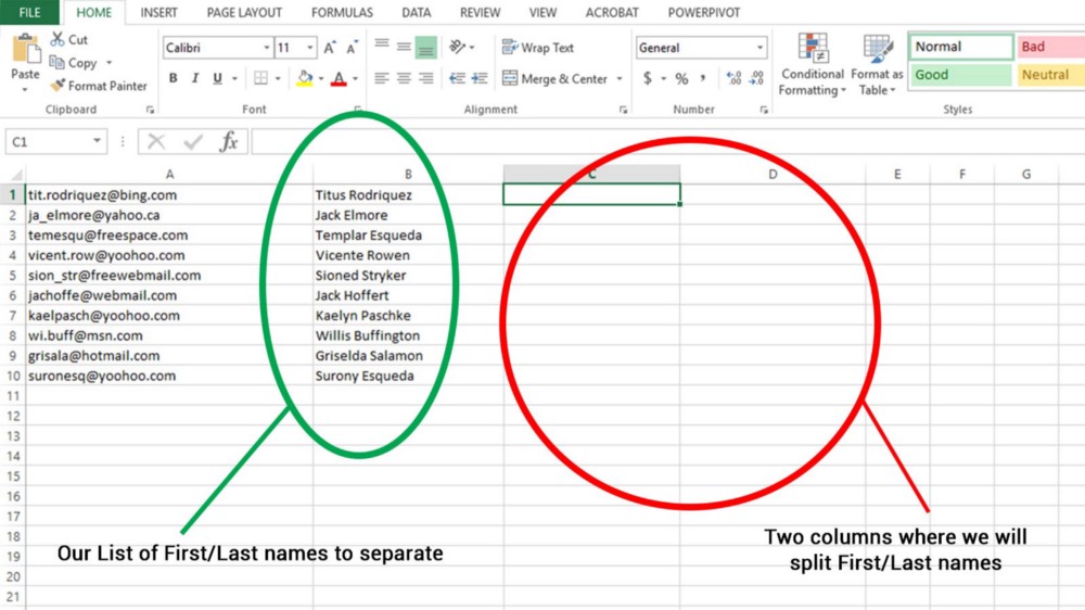
I will detail a case that frequently occurs in my work. Your experience should be modified to fit your reality. I am often tasked with sending out a newsletter or survey. The list of recipients arrives in the form of an Excel document. If I am fortunate, the document is relatively tidy and there are no spelling errors (one can dream). But, in almost all cases, the information comes in two columns — one with the email addresses, and one with the first and last name(s).
The problem? Programs and sites like Mailchimp and Surveymonkey allow you great personalization of your emails, allowing you to target and use things like the recipient’s first name, last name, or other data, but only if it is in its own column.
So, how can we clean up our first/last name problem without cutting and pasting all day? With a couple of formulas.
The Process
I will use a few illustrations to demonstrate. First, we want to make sure that the first and last names are all in one nice and near column. Make sure that there are empty columns to the right of your First/Last Name column; it isn’t necessary, but it will make your life easier.
- Now, go to the very top of your First/Last Name column, and highlight the column immediately to the right.
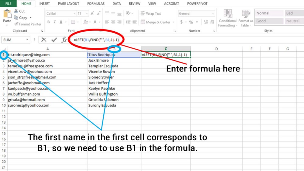
- In that first empty cell, insert the following formula:
=LEFT(A1,FIND(" ",A1,1)-1)(Note: formatting error with quotes above now fixed — copy and use!)
- Then click Enter. If all went well, you should see the first name reproduced in the empty cell where you put the formula. One important note — look at the formula, where it shows B1. This assumes that the first entry for your First/Last name column is in cell B1. If it is not, you must change it to the correct value. (B1, or whatever. See the image).
=LEFT(B1,FIND(" ",B1,1)-1)(Note: formatting error with quotes above now fixed — copy and use!)
- Then click Enter. If all went well, you should see the first name reproduced in the empty cell where you put the formula. One important note — look at the formula, where it shows B1. This assumes that the first entry for your First/Last name column is in cell B1. If it is not, you must change it to the correct value. (B1, or whatever. See the image).
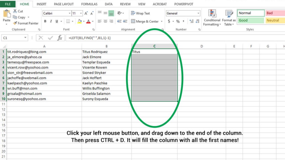
- If you enter the formula correctly and press Enter, (don’t click on a different cell while entering the formula!) you should see the first name alone in a cell. Congrats!
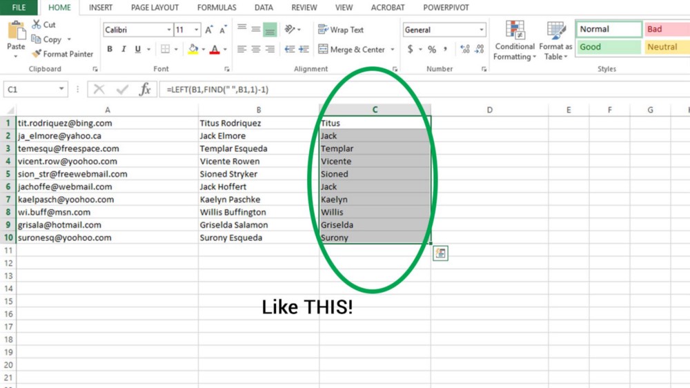
- Now, left-click on the first cell and drag the mouse down to the end of your list. You should have the whole column highlighted. Then click CTRL + D, and the column will magically fill with all the first names from your previous First/Last Name column.
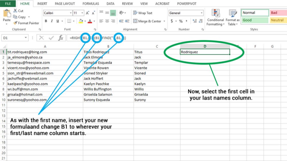
- Moving on, click on the first cell at the top of the next column (to the right of where your First Names only are. Then, enter the following formula:
=RIGHT(B1,LEN(B1)-FIND(" ",B1,1))(Note: formatting error with quotes above now fixed — copy and use!)
- Change the value B1 if necessary. Repeat the same process as above, and you should see the last name only in the first cell.
- Duplicate the process noted above, left-clicking on the first cell and dragging down and pressing CTRL + D to fill the column with Last Names only.
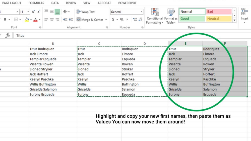
To fix this, we simply highlight the First/Last Name columns, and press CTRL + C ( or right-click and select Copy…). Then, we paste the copied columns into two different, empty columns, (it doesn’t matter which columns you paste into). However, we don’t want to paste using CTRL + V. Instead, right-click and you will see multiple paste options. Select the icon that has a 123 at the bottom. This is called Paste as Values. If you do this, you are separating the First/Last Names from the formulas, and can freely cut and paste them wherever you want in the future.
Well, that’s all here. Hope this makes your life easier. Hey, why not make my life easier and click that green heart icon at the bottom of this article, so that more people can enjoy it?